Fitting FLIM Parameters

This notebook introduces the most basic forms of using the FLIMParameters objects and tools programmatically. There is an easy-to-use graphical interface for testing many parameters in the siff-napari plugin, but that will not be covered here. Instead, look at the siff-napari documentation at - ADD LINK HERE -.

import numpy as np
import matplotlib.pyplot as plt

from siffpy.core.flim import FLIMParams


# Here I'm creating an arrival time axis.
# In principle this should be built from a
# SiffReader object, but we're just demo-ing
# here.
bin_width = 0.01
# this is in nanoseconds. 12.5 nanoseconds ~ 80 MHz laser pulse rate
tau_axis = np.arange(0, 12.5, bin_width)

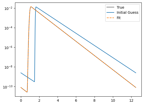
Fit a single exponential

In this first example, we generate an arrival time distribution corresponding to a single exponential arrival time distribution convolved with a Gaussian IRF. This is as simple as

\[\begin{split}F(t; \tau, \mu, \sigma) = \text{exp}\left(\frac{(t-\mu)^2}{\sigma^2}\right) * \text{exp}(-t/\tau) \\ F(t; \tau, \mu, \sigma) = \sqrt{\frac{\pi\sigma^2}{2\tau^2}}\exp\left(\frac{\sigma^2}{2\tau^2}\right)\text{erfc} \left(\frac{1}{\sqrt{2}}\left(\frac{\sigma}{\tau} - \frac{x-\mu}{\sigma}\right) \right) \exp\left(-\frac{x-\mu}{\tau}\right)\end{split}\]

Here $\tau$ is the decay of the exponential, $\mu$ is the mean delay of the laser pulse + travel of the photon to the detector, and $\sigma$ is a measure of the ballistic spread in arrival times. $*$ denotes the convolutional operator, not multiplication.

from scipy.optimize import minimize
from siffpy.core.flim.flimparams import multi_exponential_pdf_from_params

def objective(params, tau_axis, data):
    return np.sum(
        (
            (multi_exponential_pdf_from_params(tau_axis, params)[1:] - data[1:])**2
            / data[1:]
        )
    )

# There are many ways to instantiate a FLIMParams object.
# In this example, we use a dictionary to specify the parameters.
monoexp = FLIMParams.from_dict(
    dict(
        exps = [
            dict(tau = 0.6, fraction = 1.0, units = 'nanoseconds'),
        ],
        irf = dict(tau_g = 0.05, mean = 1.0, units = "nanoseconds")
    )
)

print(monoexp.noise)

data = monoexp.pdf(tau_axis)

# A not-very-good guess.
init_guess = np.array((0.7, 1.0, 1.6, 0.02)) # tau f1 irf_mean, irf_sigma

plt.semilogy(
    tau_axis,
    data,
    label = 'True',
    color = '#666666'
)

plt.semilogy(
    tau_axis,
    multi_exponential_pdf_from_params(tau_axis, init_guess),
    label = 'Initial Guess',
)


res = monoexp.fit_params_to_data(
    data,
    init_guess,
    x_range = tau_axis,
)

plt.semilogy(
    tau_axis,
    multi_exponential_pdf_from_params(tau_axis, res.x),
    label = 'Fit',
    linestyle = '--',
)

plt.legend()

print(f"{res.niter} iterations : {res.x}")

# Looks great! The green dashed line basically exactly covers the blue

0.0
90 iterations : [0.6  1.   1.   0.05]

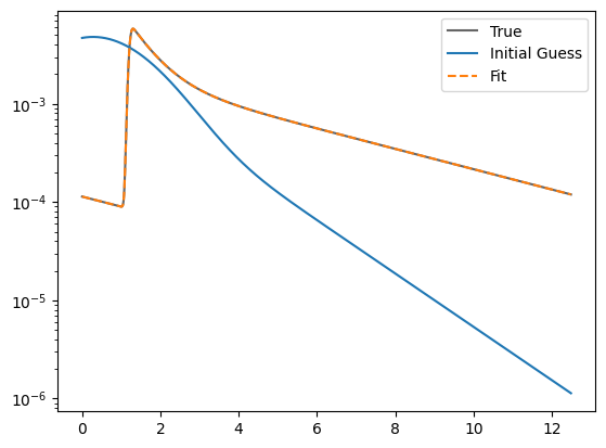
_images/multi_pulse_flim_notebook_3_1.png

Fitting two exponentials

Now we’ll generate data from a distribution with two exponentials in a mixture. This is as before, but now there are two exponentials, each contributing to some fraction of the signal:

\[F(t) = f_1 F(t; \tau_1, \sigma, \mu) + f_2 F(t; \tau_2, \sigma, \mu)\]

with $f_1 + f_2 = 1$. We’ll also, just for the sake of documentation, show how to initialize a FLIMParams from the siffpy classes of FLIMParameters

from siffpy.core.flim import Exp, Irf
biexponential = FLIMParams(
    Exp(tau = 0.6, fraction = 0.3, units = 'nanoseconds'),
    Exp(tau = 4.2, fraction = 0.7, units = 'nanoseconds'),
    Irf(tau_g = 0.05, mean = 1.2, units = "nanoseconds")
)

data = biexponential.pdf(tau_axis)

# A quite bad guess!
init_guess = np.array((0.2, 0.8, 1.6, 0.2, 0.0, 1.25)) # tau f1 irf_mean, irf_sigma

res = biexponential.fit_params_to_data(
    data,
    init_guess,
    x_range = tau_axis,
)

plt.semilogy(
    tau_axis,
    data,
    label = 'True',
    color = '#666666'
)

plt.semilogy(
    tau_axis,
    multi_exponential_pdf_from_params(tau_axis, init_guess),
    label = 'Initial Guess',

)

plt.semilogy(
    tau_axis,
    multi_exponential_pdf_from_params(tau_axis, res.x),
    label = 'Fit',
    linestyle = '--',
)

plt.legend()

print(f"{res.niter} iterations. {res.x}")

77 iterations. [0.60000114 0.30000055 4.20000429 0.69999945 1.19999999 0.05000003]

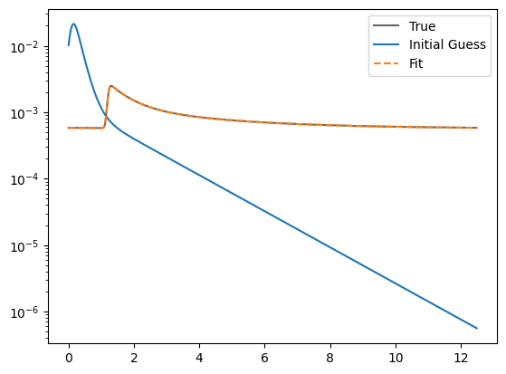
_images/multi_pulse_flim_notebook_5_1.png

Add background noise

Typically our data comes with some background noise that is independent of the laser pulse, e.g. background illumination, visual stimuli. We can also fit keeping that fact in mind.

In this case, we’ll make the noise very strong (half of our “signal” is actually noise!). This is not a problem. This corresponds to the model

\[F(t) = f_1 F(t; \tau_1, \mu, \sigma) + f_2 F(t; \tau_2, \mu, \sigma) + \epsilon\]

where $ f_1 + f2 + :raw-latex:`epsilon `= 1$ (keeping this a probability distribution)

biexponential = FLIMParams(
    Exp(tau = 0.6, fraction = 0.3, units = 'nanoseconds'),
    Exp(tau = 4.2, fraction = 0.7, units = 'nanoseconds'),
    Irf(tau_g = 0.05, mean = 1.2, units = "nanoseconds"),
    noise = 0.5,
)

data = biexponential.pdf(tau_axis)

init_guess = np.array((0.2, 0.8, 1.6, 0.2, 0.05, 1.25, 0.0)) # tau f1 ... , irf_mean, irf_sigma, noise

def noisy_objective(params, tau_axis, data):
    return np.sum(
        (
            (
                np.ones_like(tau_axis[1:])*params[-1]/len(tau_axis) # noise
                + (1-params[-1])*multi_exponential_pdf_from_params(tau_axis, params[:-1])[1:]
                - data[1:]
            )**2
            / data[1:]
        )
    )

res = biexponential.fit_params_to_data(
    data,
    init_guess,
    x_range = tau_axis,
)

plt.semilogy(
    tau_axis,
    data,
    label = 'True',
    color = '#666666',
)

plt.semilogy(
    tau_axis,
    multi_exponential_pdf_from_params(tau_axis, init_guess[:-1]),
    label = 'Initial Guess',
)

plt.semilogy(
    tau_axis,
    (
        res.x[-1]*np.ones_like(tau_axis)/len(tau_axis) # noise
        + (1-res.x[-1])*multi_exponential_pdf_from_params(tau_axis, res.x[:-1])
    ),
    label = 'Fit',
    linestyle = '--',
)

plt.legend()

print(f"{res.niter} iterations. {res.x}.")

538 iterations. [0.60000249 0.30000064 4.20003483 0.69999936 1.19999993 0.05000002
 0.49999848].

_images/multi_pulse_flim_notebook_7_1.png

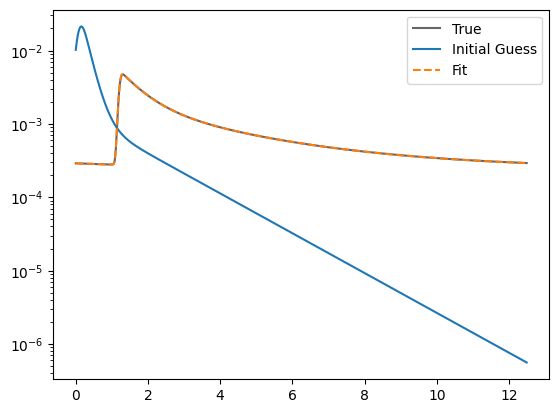
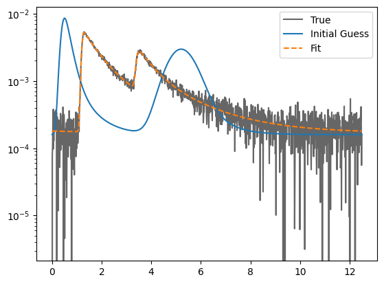
Pushing it to the limit

This has got to be much harder: 70% of the signal is noise, and there are now THREE exponentials producing the data, each approximately to the same extent! Okay… so this one doesn’t do quite as well. Hopefully you never have data quite this messy. The curve itself looks pretty okay, but if you look at the actual values for tau and the fractions… it could be better.

In general, FLIMParams objects will fit the model

\[F(t) = \epsilon + \displaystyle\sum_{i=1}^{N}f_i F(t; \tau_i, \mu, \sigma)\]

with the constraints

\[\begin{split}\tau_i < \tau_j \hspace{6mm} \forall i<j \\ \sum_{i=1}^{n}f_i = 1\end{split}\]

triexponential = FLIMParams.from_dict(
    dict(
        exps = [
            dict(tau = 0.6, fraction = 0.3, units = 'nanoseconds'),
            dict(tau = 2.1, fraction = 0.3, units = 'nanoseconds'),
            dict(tau = 4.2, fraction = 0.4, units = 'nanoseconds'),
        ],
        irf = dict(tau_g = 0.05, mean = 1.2, units = "nanoseconds"),
        noise = 0.7,
    )
)

data = triexponential.pdf(tau_axis)

init_guess = np.array((0.2, 0.8, 0.4, 0.0, 1.6, 0.2, 0.05, 0.1, 0.4)) # tau f1 ... , irf_mean, irf_sigma, noise

def noisy_objective(params, tau_axis, data):
    return np.sum(
        (
            (
                np.ones_like(tau_axis[1:])*params[-1]/len(tau_axis) # noise
                + (1-params[-1])*multi_exponential_pdf_from_params(tau_axis, params[:-1])[1:]
                - data[1:]
            )**2
        ) / data[1:]
    )

res = minimize(
    noisy_objective,
    init_guess,
    args = (tau_axis, data),
    bounds = triexponential.bounds,
    constraints = triexponential.constraints,
    method = 'trust-constr',
)

# res = triexponential.fit_params_to_data(
#     data,
#     init_guess,
#     x_range = tau_axis,
# )

plt.semilogy(
    tau_axis,
    data,
    label = 'True',
    color = '#666666',
)

plt.semilogy(
    tau_axis,
    multi_exponential_pdf_from_params(tau_axis, init_guess[:-1]),
    label = 'Initial Guess',
)

plt.semilogy(
    tau_axis,
    (
        res.x[-1]*np.ones_like(tau_axis)/len(tau_axis) # noise
        + (1-res.x[-1])*multi_exponential_pdf_from_params(tau_axis, res.x[:-1])
    ),
    label = 'Fit',
    linestyle = '--',
)

plt.legend()

print(f"{res.niter} iterations. {res.x}")

1000 iterations. [0.60509998 0.30504688 2.41324031 0.42841357 5.07295958 0.26653955
 1.19996303 0.04998284 0.69887643]

_images/multi_pulse_flim_notebook_9_1.png

Reducing the noise a little gives us a much faster-converging estimate

triexponential = FLIMParams.from_dict(
    dict(
        exps = [
            dict(tau = 0.6, fraction = 0.3, units = 'nanoseconds'),
            dict(tau = 2.1, fraction = 0.3, units = 'nanoseconds'),
            dict(tau = 4.2, fraction = 0.4, units = 'nanoseconds'),
        ],
        irf = dict(tau_g = 0.05, mean = 1.2, units = "nanoseconds"),
        noise = 0.3,
    )
)

data = triexponential.pdf(tau_axis)

init_guess = np.array((0.2, 0.8, 0.4, 0.0, 1.6, 0.2, 0.05, 0.1, 0.4)) # tau f1 ... , irf_mean, irf_sigma, noise

def noisy_objective(params, tau_axis, data):
    return np.sum(
        (
            (
                np.ones_like(tau_axis[1:])*params[-1]/len(tau_axis) # noise
                + (1-params[-1])*multi_exponential_pdf_from_params(tau_axis, params[:-1])[1:]
                - data[1:]
            )**2
            / data[1:]
        )
    )

# res = minimize(
#     noisy_objective,
#     init_guess,
#     args = (tau_axis, data),
#     bounds = triexponential.bounds,
#     constraints = triexponential.constraints,
#     method = 'trust-constr',
# )

res = triexponential.fit_params_to_data(
    data,
    init_guess,
    x_range = tau_axis,
)

plt.semilogy(
    tau_axis,
    data,
    label = 'True',
    color = '#666666',
)

plt.semilogy(
    tau_axis,
    multi_exponential_pdf_from_params(tau_axis, init_guess[:-1]),
    label = 'Initial Guess',
)

plt.semilogy(
    tau_axis,
    (
        res.x[-1]*np.ones_like(tau_axis)/len(tau_axis) # noise
        + (1-res.x[-1])*multi_exponential_pdf_from_params(tau_axis, res.x[:-1])
    ),
    label = 'Fit',
    linestyle = '--',
)

plt.legend()

print(f"{res.niter} iterations. {res.x}")

910 iterations. [0.60045092 0.30047337 2.12496322 0.30890674 4.24453728 0.39061989
 1.19999659 0.0499987  0.29979893]

_images/multi_pulse_flim_notebook_11_1.png

Multiple pulses

Let’s make things a little harder yet again. Now we’re going to model a system in which there are multiple fluorophores with different emission spectra, and excited by TWO laser sources. Both laser sources excite both fluorophores (with different efficacy), and our job will be to wrest the true signal out of this mess.

This signal corresponds to the equations

\[\begin{split}F(t) = \epsilon + \displaystyle\sum_{l=1}^{N_l}\displaystyle\sum_{i=1}^{N_s}f_i\varphi_l F(t; \tau_i, \mu_{l}, \sigma_{l}) \\\end{split}\]

with the constraints $$

:raw-latex:`\sum`_{l} :raw-latex:`\varphi`l = 1 \ :raw-latex:`sum`{i} f_i = 1 \ :raw-latex:`\tau`_i < :raw-latex:`\tau`_j :raw-latex:`\hspace{6mm}` :raw-latex:`forall `i<j \ $$

where now $l$ is indexing over the laser pulses and $i$ is indexing over fluorophore states.

We have a separate class for this specific instance: the MultiPulseFLIMParam. This section of the code will first solve the problem the hard way (with regular FLIMParams) to build intuition and then will use the MultiPulseFLIMParam. Part of the reason this section is structured this way is that I’m building the MultiPulseFLIMParam class while I write it! So this may be revised in the future…

So our tricky distribution was no problem for the solver.

green_fluorophore_pulse_one = FLIMParams.from_dict(
    dict(
        exps = [
            dict(tau = 0.6, fraction = 0.5, units = 'nanoseconds'),
            dict(tau = 2.1, fraction = 0.5, units = 'nanoseconds'),
        ],
        irf = dict(tau_g = 0.05, mean = 1.2, units = "nanoseconds"),
        noise = 0.2,
    )
)

green_fluorophore_pulse_two = FLIMParams.from_dict(
    dict(
        exps = [
            dict(tau = 0.6, fraction = 0.5, units = 'nanoseconds'),
            dict(tau = 2.1, fraction = 0.5, units = 'nanoseconds'),
        ],
        irf = dict(tau_g = 0.07, mean = 3.4, units = "nanoseconds"),
        noise = 0.2,
    )
)

frac_pulse_one = 0.7
frac_pulse_two = 1 - frac_pulse_one

data = (
    frac_pulse_one*green_fluorophore_pulse_one.pdf(tau_axis)
    + frac_pulse_two*green_fluorophore_pulse_two.pdf(tau_axis)
)

from scipy.optimize import Bounds, LinearConstraint, minimize

def noisy_multipulse_objective(params, tau_axis, data):
    """
    Params are now of length 1x exp + 2xirf parameters plus one frac for each irf plus one noise parameter
    """
    noise = params[-1]
    return np.sum(
        (
            np.ones_like(tau_axis[1:])*noise/len(tau_axis) # noise
            + (1-noise)*(
                params[-5]*multi_exponential_pdf_from_params(tau_axis, params[:-5])[1:]+
                params[-2]*multi_exponential_pdf_from_params(tau_axis, np.append(params[:4], params[-4:-2]))[1:]
            )
            - data[1:]
        )**2
    )/np.sum(data[1:])


init_guess = np.array((0.2, 0.8, 0.7, 0.2, 0.4, 0.1, 0.5, 5.0, 0.5, 0.5, 0.2)) # tau f1 ... , irf_mean, irf_sigma, frac_irf_1, irf_mean_2, irf_sigma_2, frac_irf_2, noise

data = (
    frac_pulse_one*green_fluorophore_pulse_one.pdf(tau_axis)
    + frac_pulse_two*green_fluorophore_pulse_two.pdf(tau_axis)
) + 1e-4*np.random.randn(len(tau_axis))
multi_pulse_bounds = Bounds(
        lb = [0, 0, 0, 0, 0, 0, 0, 0, 0, 0, 0],
        ub = [np.inf, 1, np.inf, 1, np.inf, np.inf, 1, np.inf, np.inf, 1, 1],
)

multi_pulse_constraints = [
    LinearConstraint( # sum of fractions = 1
        A = [0,1,0,1,0,0,0,0,0,0,0],
        lb = 1,
        ub = 1,
    ),
    LinearConstraint( # sum of irf_fractions = 1
        A = [0,0,0,0,0,0,1,0,0,1,0],
        lb = 1,
        ub = 1,
    ),
    LinearConstraint( # tau_1 < tau_2
        A = [1,0,-1,0,0,0,0,0,0,0,0],
        lb = -np.inf,
        ub = 0,
    ),
    LinearConstraint( # irf_1 < irf_2
        A = [0,0,0,0,1,0,0,-1,0,0,0],
        lb = -np.inf,
        ub = -0.1,
    ),
]

print(len(multi_pulse_bounds.lb), len(init_guess))


res = minimize(
    noisy_multipulse_objective,
    init_guess,
    args = (tau_axis, data),
    bounds = multi_pulse_bounds,
    constraints = multi_pulse_constraints,
    method = 'trust-constr',
)

plt.semilogy(
    tau_axis,
    data,
    label = 'True',
    color = '#666666',
)

plt.semilogy(
    tau_axis,
    (
        init_guess[-1]*np.ones_like(tau_axis)/len(tau_axis) # noise
        +(1-init_guess[-1])*(
            init_guess[-5]*multi_exponential_pdf_from_params(tau_axis, init_guess[:-5])+
            init_guess[-2]*multi_exponential_pdf_from_params(tau_axis, np.append(init_guess[:4], init_guess[-4:-2]))
        )
    ),
    label = 'Initial Guess',
)

plt.semilogy(
    tau_axis,
    (
        res.x[-1]*np.ones_like(tau_axis)/len(tau_axis) # noise
        +(1-res.x[-1])*(
            res.x[-5]*multi_exponential_pdf_from_params(tau_axis, res.x[:-5])+
            res.x[-2]*multi_exponential_pdf_from_params(tau_axis, np.append(res.x[:4], res.x[-4:-2]))
        )
    ),
    label = 'Fit',
    linestyle = '--',
)

plt.legend()

print(f"{res.niter} iterations. {res.x}")

11
iterations. [0.59441365 0.48866273 1.90361903 0.51133727 1.19906974 0.05014742
69620238 3.40056867 0.06931414 0.30379762 0.21359188]

_images/multi_pulse_flim_notebook_14_1.png

Now we can try it with the `MultiPulseFLIMParams`

These use a different type of Irf object: the FractionalIrf, which allows a different fraction of the fluorescence to come from each pulse. You can actually just pass in regular Irf objects and they will be converted into FractionalIrfs with each getting an equal fraction.

from siffpy.core.flim import Exp
from siffpy.core.flim.multi_pulse import FractionalIrf, MultiPulseFLIMParams
import matplotlib.pyplot as plt
mpfp = MultiPulseFLIMParams(
    Exp(tau = 0.1, fraction = 0.25, units = 'nanoseconds'),
    Exp(tau = 1.4, fraction = 0.75, units = 'nanoseconds'),
    FractionalIrf(tau_g = 0.05, mean = 0.4, frac = 0.37, units = "nanoseconds"),
    FractionalIrf(tau_g = 0.07, mean = 5.5, frac = 0.63, units = "nanoseconds"),
    noise = 0.2
)

print(mpfp.params)

data = (
    frac_pulse_one*green_fluorophore_pulse_one.pdf(tau_axis)
    + frac_pulse_two*green_fluorophore_pulse_two.pdf(tau_axis)
) + (1e-1/len(tau_axis))*np.random.randn(len(tau_axis))

res = mpfp.fit_params_to_data(
    data,
    #initial_guess=init_guess,
    x_range = tau_axis,
)

plt.semilogy(
    tau_axis,
    data,
    label = 'True',
    color = '#666666',
)

plt.semilogy(
    tau_axis,
    mpfp.pdf(tau_axis),
    label = 'Fit',
    linestyle = '--',
)

plt.legend()

[Exp
    UNITS: FlimUnits.NANOSECONDS
    tau : 0.1
    frac : 0.25
, Exp
    UNITS: FlimUnits.NANOSECONDS
    tau : 1.4
    frac : 0.75
, MultiIrf([FractionalIrf
    UNITS: FlimUnits.NANOSECONDS
    tau_offset : 0.4
    tau_g : 0.05
    frac : 0.37
, FractionalIrf
    UNITS: FlimUnits.NANOSECONDS
    tau_offset : 5.5
    tau_g : 0.07
    frac : 0.63
])]

<matplotlib.legend.Legend at 0x177b7f190>

_images/multi_pulse_flim_notebook_16_2.png

from IPython.display import display, Latex
param_dict = triexponential.to_dict()
irfstr = f"\\text{{exp}}\\left(\\frac{{(t - {param_dict['irf']['tau_offset']})^2}}{{{param_dict['irf']['tau_g']}^2}}\\right)"
display(Latex(f"$${irfstr}$$"))

\[\text{exp}\left(\frac{(t - 1.1999965897342781)^2}{0.04999870276961093^2}\right)\]

Multiple fluorophores and multiple pulses

Now it gets even crazier – often we’re using two laser pulses because we have multiple fluorophores, each differentially excitable by different lasers. Similarly, we can image with multiple fluorophores in the same channel even with only one pulse. For this, we have a more complex set of contingencies; some parameters are shared across channels, and we need a MultiFluorophoreFLIMParams, which gets even more complicated, because it combines several MultiFLIMParams. The channel itself will be composed of many fluorophores sharing MultiIrfs, a common noise term, and a summed fraction of fluorophores, each having their own fractions. Here goes nothing…

The final boss: multiple channels, multiple fluorophores, multiple pulses

Typically you might want to fit your FLIM channels separately – often we have one channel for one fluorophore, and another channel for the other fluorophore. But unfortunately, sometimes there’s bleedthrough, and our signal gets contaminated by the other fluorophore. Our job is to sort these out, aided by the parameters that are shared across channels. Each fluorophore’s $\tau$ and $f$ parameters should be shared across channels and each IRF should be shared across channels – it’s just that each fluorophore’s state needs a weight for each channel (meaning that there is $n_{\text{channels}}-1$ free parameters per fluorophore state introduced by the presence of multiple channels, I think – maybe not quite right).